Intro to Tidyverse
Introduction to the Tidyverse
Tidy data is data that exists in a controlled and structured format that allows for consistent manipulation. It is good practice to keep your data clean and tidy before working with it. As they say: garbage in, garbage out.
If you want more information regarding what “tidy” data means you can read more about it here: http://vita.had.co.nz/papers/tidy-data.html
You can also reference the free book by Hadley Wickhman called “R for Data Science”. The entire book is found here: https://r4ds.had.co.nz/tidy-data.html
NYC Flights Data
We will start by installing the NCY Flights Package that contains the data that we will need for this demo.
This package is a collection of datasets compiled by Hadley Wickham, author of many of the Tidyverse Packages we will look at. We will be using this dataset because it contains a variety of variables that will allow us to explore more functions than a basic numerical table with integers and factors. If you want more information on this package you can load the help file in R or see https://github.com/hadley/nycflights13.
## -- Attaching packages --------------------------------------------------------- tidyverse 1.2.1 --
## v ggplot2 3.0.0     v purrr   0.2.5
## v tibble  1.4.2     v dplyr   0.7.6
## v tidyr   0.8.1     v stringr 1.3.1
## v readr   1.1.1     v forcats 0.3.0
## -- Conflicts ------------------------------------------------------------ tidyverse_conflicts() --
## x dplyr::filter() masks stats::filter()
## x dplyr::lag()    masks stats::lag()
While the nycflights13 package contains several separate datasets, we will specifically be looking at “flights”. Start by loading this data and exploring the structure.
data("flights")
head(flights)
## # A tibble: 6 x 19
##    year month   day dep_time sched_dep_time dep_delay arr_time
##   <int> <int> <int>    <int>          <int>     <dbl>    <int>
## 1  2013     1     1      517            515         2      830
## 2  2013     1     1      533            529         4      850
## 3  2013     1     1      542            540         2      923
## 4  2013     1     1      544            545        -1     1004
## 5  2013     1     1      554            600        -6      812
## 6  2013     1     1      554            558        -4      740
## # ... with 12 more variables: sched_arr_time <int>, arr_delay <dbl>,
## #   carrier <chr>, flight <int>, tailnum <chr>, origin <chr>, dest <chr>,
## #   air_time <dbl>, distance <dbl>, hour <dbl>, minute <dbl>,
## #   time_hour <dttm>
colnames(flights)
##  [1] "year"           "month"          "day"            "dep_time"
##  [5] "sched_dep_time" "dep_delay"      "arr_time"       "sched_arr_time"
##  [9] "arr_delay"      "carrier"        "flight"         "tailnum"
## [13] "origin"         "dest"           "air_time"       "distance"
## [17] "hour"           "minute"         "time_hour"
Using dplyr for Data Manipulation on Columns
dplyr is a package contained in the Tidyverse and contains functions that you will need for performing a number of standard manipulations on data. This package was loaded with the tidyverse, so no need to load it separately.
select allows you to perform manipulations on columns.
Lets get rid of some columns we don’t want using dplyr’s select function. Only keep columns that have “time” in the name.
flight_names = select(flights, contains("time"))
head(flight_names)
## # A tibble: 6 x 6
##   dep_time sched_dep_time arr_time sched_arr_time air_time
##      <int>          <int>    <int>          <int>    <dbl>
## 1      517            515      830            819      227
## 2      533            529      850            830      227
## 3      542            540      923            850      160
## 4      544            545     1004           1022      183
## 5      554            600      812            837      116
## 6      554            558      740            728      150
## # ... with 1 more variable: time_hour <dttm>
colnames(flight_names)
## [1] "dep_time"       "sched_dep_time" "arr_time"       "sched_arr_time"
## [5] "air_time"       "time_hour"
More: Try and insert any other character string of interest instead of “time”
You can also select columns that end in a particular string. Lets try to only select columns that end in “ay”.
flight_ay = select(flights, ends_with("ay"))
colnames(flight_ay)
## [1] "day" "dep_delay" "arr_delay"
Using starts_with(“”) instead of ends_with(“”) we are able to select those that begin with a specific string.
flight_de = select(flights, starts_with("de"))
colnames(flight_de)
## [1] "dep_time" "dep_delay" "dest"
Select will also allow you to select specific columns by name. While this can be a slower method, it is often neccessary.
flight_set = select(flights, one_of(c("year", "month", "day", "arr_time")))
colnames(flight_set)
## [1] "year" "month" "day" "arr_time"
The inverse of selecting specific columns is dropping them by name. This can be achieved by placing a - in front of the named column to be dropped.
flight_minus = select(flights, -dep_delay)
colnames(flight_minus)
##  [1] "year"           "month"          "day"            "dep_time"
##  [5] "sched_dep_time" "arr_time"       "sched_arr_time" "arr_delay"
##  [9] "carrier"        "flight"         "tailnum"        "origin"
## [13] "dest"           "air_time"       "distance"       "hour"
## [17] "minute"         "time_hour"
One of the powerful things about this function is that you can simply place a - in front of other commands that we already looked at to remove them by these criteria.
flight_de_minus = select(flights, -starts_with("de"))
colnames(flight_de_minus)
##  [1] "year"           "month"          "day"            "sched_dep_time"
##  [5] "arr_time"       "sched_arr_time" "arr_delay"      "carrier"
##  [9] "flight"         "tailnum"        "origin"         "air_time"
## [13] "distance"       "hour"           "minute"         "time_hour"
dplyr for Row Manipulation
While the select fuction is useful when working with column selection, sometimes you need to select a subset of rows. To do that we make use of filter().
select() is for columns, filter() is for rows
Lets look at only flights from United Airlines (UA)
ua_flights = filter(flights, carrier == "UA")
If you have a group of variables that you would like to use for row selection we can do that as well. First we will assign a variable named “group” that contains our character strings of interest. Then we can select all the rows that match this by defining them as members in our group.
group = c("UA", "AA" , "DL")
ua_group_flights = filter(flights, carrier %in% group)
colnames(ua_group_flights)
##  [1] "year"           "month"          "day"            "dep_time"
##  [5] "sched_dep_time" "dep_delay"      "arr_time"       "sched_arr_time"
##  [9] "arr_delay"      "carrier"        "flight"         "tailnum"
## [13] "origin"         "dest"           "air_time"       "distance"
## [17] "hour"           "minute"         "time_hour"
Help: if this is unclear, read the command as: the variable ua_group_flights is a filtered selection from the dataset flights. Filtering is performed on the column named carrier for all items in the variable group.
When working with columns we used - to exclude from our selection, when working with rows ! is used instead. != is a logical operator that can be read as “not equal to”
ua_minus_flights = filter(flights, carrier != "UA")
colnames(ua_minus_flights)
##  [1] "year"           "month"          "day"            "dep_time"
##  [5] "sched_dep_time" "dep_delay"      "arr_time"       "sched_arr_time"
##  [9] "arr_delay"      "carrier"        "flight"         "tailnum"
## [13] "origin"         "dest"           "air_time"       "distance"
## [17] "hour"           "minute"         "time_hour"
These functions thus far are powerful, fast, and commonly used. However, as scientists most of our data is numerical in nature. Thus we need to filter based on numerical criteria as well.
In this example months are reported as numbers between 1-12 so the numbers represent categorical variables. However these functions can be applied in other more biological situations such as:
- select mice of interest based on their weight or age
- select data based on time
- make selections above or below a set threshold
To select just those flights from February, use month ==2.
feb_flight = filter(flights, month == 2)
half_flight = filter (flights, month <= 6)
The Pipe Operator
Let’s be real.. code is for computers to read, not humans. To improve the readability of code and prevent complicated nested functions we use the pipe operator: %>% This technically comes from the magrittr package, but is loaded with the Tidyverse. When using the pipe operator functions are applied sequentially in a top down fashion. Meaning in the example below, select is applied before filter. While it doesn’t make a difference in this example, order can be important depending on the situation.
flight_set = flights %>%
  select(-dep_delay) %>%
  filter(month == 2)
colnames(flight_set)
##  [1] "year"           "month"          "day"            "dep_time"
##  [5] "sched_dep_time" "arr_time"       "sched_arr_time" "arr_delay"
##  [9] "carrier"        "flight"         "tailnum"        "origin"
## [13] "dest"           "air_time"       "distance"       "hour"
## [17] "minute"         "time_hour"
Now we just have everything except dep_delay in the month of febuary (2) as a new variable named flight_set.
Descriptive Statistics using Summary
This is where a lot of the data everyone wants to access quicklly will come from.
As a side note for a later discussion, the tidyverse makes use of a data.frame structure called the tibble. Think of it as data.table 2.0 that has all the good stuff and a shiny new coat of paint. Our flights data and all the data in this example is in a tibble. One of the improvements on the standard data frame that is implemented in a tibble is that strings are not automatically converted to factors. While this might not mean much to you now, I promise this will not be the first time you deal with the complications regarding “strings as factors”.
As such, before we can group our air carriers for data summary, we actually do need to convert them to factors. This way R will recognize them as factors and not simply a vector containing duplicated strings.
flight_set$carrier = as.factor(flight_set$carrier)
Here we are going to create a new variable called mean_dist. This will use the flight_set data that we created earlier. We then tell R to group the data by carrier and calculate the mean distance traveled from the distance column for each group. This mean will then be output to a newly named column in mean_dist called distance_avg.
mean_dist = flight_set %>%
  group_by(carrier) %>%
  summarise(distance_avg = mean(distance))

mean_dist
## # A tibble: 15 x 2
##    carrier distance_avg
##    <fct>          <dbl>
##  1 9E              468.
##  2 AA             1350.
##  3 AS             2402
##  4 B6             1057.
##  5 DL             1227.
##  6 EV              525.
##  7 F9             1620
##  8 FL              691
##  9 HA             4983
## 10 MQ              565.
## 11 UA             1436.
## 12 US              527.
## 13 VX             2493.
## 14 WN              950.
## 15 YV              229
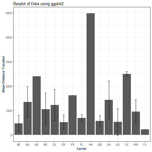
Make a plot you would be proud to show at lab meeting
Here we will make a few modifications so that we have the standard deviation as well as the mean. You are scientists, shame on you if you don’t add error bars.
mean_dist = flight_set %>%
  group_by(carrier) %>%
  summarise(distance_avg = mean(distance), sd = sd(distance))
Without much additional explanation here, lets plot this out using ggplot2.
ggplot(mean_dist, aes(x= mean_dist$carrier, y =  mean_dist$distance_avg)) +
  geom_bar(stat = "identity") +
  geom_errorbar(aes(ymin=distance_avg-sd, ymax=distance_avg+sd),
                size=.3,    # Thinner lines
                width=.2,
                position=position_dodge(.9)) +
  ylab("Mean Distance Traveled") +
  xlab("Carrier") +
  labs(title = "Barplot of Data using ggplot2") +
  theme_bw()